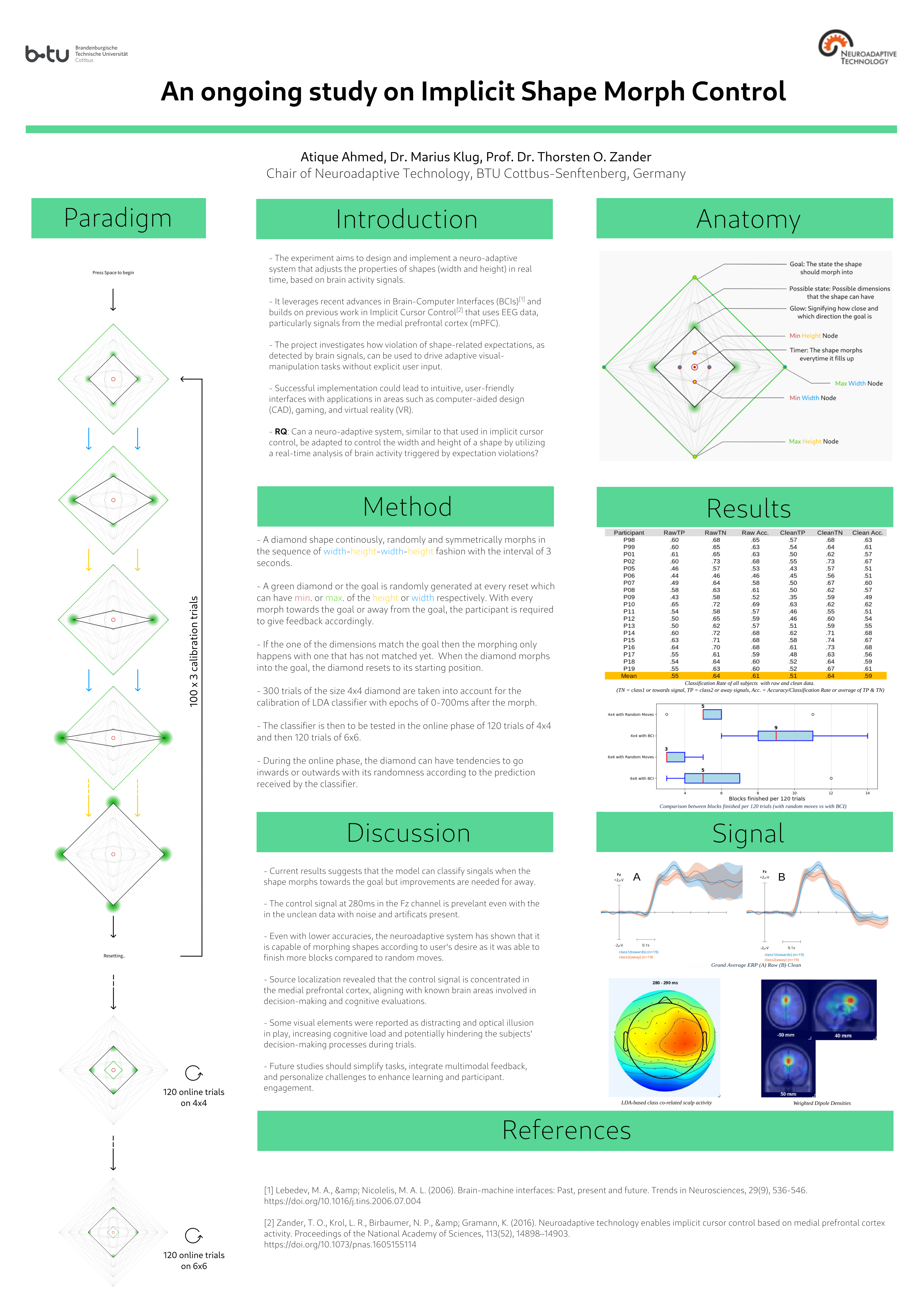
TLDR Poster #
(Open first, then right click and open image in new tab for clarity)
Abstract #
Recent advances in brain-computer interfaces (BCIs) have enabled the development of systems that adapt in real time to the user’s cognitive states. Building on the concept of implicit cursor control (ICC), this study investigates the feasibility of a neuroadaptive system that regulates the width and height of a shape based on real-time analysis of brain activity, specifically targeting the medial prefrontal cortex (mPFC) responses to expectation violations. In a controlled experimental setting, 19 healthy volunteers wear a 64-channel electroencephalography (EEG) headset while observing a dynamically changing diamond shape on a screen. The experiment consists of a calibration phase — where a linear discriminant analysis (LDA) classifier is trained using error-related brain potentials — and an online phase, during which the shape’s parameters are modulated in response to the classifier’s outputs. This approach aims to deepen our understanding of the neural correlates of shape perception and manipulation while paving the way for more intuitive human-computer interfaces in areas such as computer-aided design, gaming, and virtual reality. The expected outcomes include not only enhanced insights into the use of EEG signals for adapting interface behavior but also the establishment of a novel framework for neuroadaptive control in dynamic visual environments.
1.1 Introduction #
Artificial Intelligence (AI) is a rapidly evolving field that focuses on creating systems capable of performing tasks that typically require human intelligence. These tasks include reasoning, learning, problem-solving, perception, and language understanding. These technologies are present in various sectors, from healthcare and finance to entertainment and transportation, significantly transforming how we interact with the world. In healthcare, for instance, AI applications include diagnostic tools that analyze medical images, predictive analytics for patient outcomes, and personalized treatment plans. AI algorithms can detect diseases such as cancer at earlier stages than traditional methods, improving patient prognosis (Esteva et al., 2019). In the financial sector, AI is utilized for fraud detection, risk assessment, and algorithmic trading. Machine learning models analyze transaction patterns to identify anomalies, thereby enhancing security and efficiency (Chen et al., 2020). The entertainment industry has also been transformed through AI, which enables personalized content recommendations, automated content creation, and enhanced user experiences. Streaming platforms like Netflix and Spotify leverage AI algorithms to suggest content based on user preferences, creating a more engaging experience (Gomez-Uribe & Hunt, 2016). Transportation has seen significant advancements with the integration of AI in autonomous vehicles, traffic management systems, and logistics optimization. Self-driving cars utilize AI to navigate complex environments, making real-time decisions based on sensor data (Goodall, 2014). The applications of AI in 3D modeling extend across multiple industries. In architecture and construction, AI tools can generate building designs that optimize space utilization and energy efficiency. In the gaming and entertainment industry, AI is used to create realistic 3D environments and characters. Procedural generation techniques, powered by AI, allow for the automatic creation of vast and intricate game worlds, reducing the time and effort required by artists and developers (Shaker et al., 2016). Additionally, AI can enhance character animation by predicting movements and generating realistic behaviors based on physical simulations.
As AI continues to advance, its integration with Brain-Computer Interfaces (BCI) presents exciting opportunities for enhancing human-computer interaction (HCI). This intersection of AI and BCI is paving the way for innovative applications that can significantly improve the quality of life for individuals with disabilities and enhance human capabilities (Abdulkader et al, 2015).
BCIs are systems that decode brain activity and translate it into commands for external devices. They can be classified into two main types: invasive and non-invasive. Invasive BCIs involve surgical implantation of electrodes directly into the brain, providing high-resolution signals but carrying risks associated with surgery. Non-invasive BCIs, on the other hand, utilize external sensors, such as electroencephalography (EEG), to capture brain activity without the need for surgical procedures. While non-invasive methods may offer lower signal quality, they are safer and more accessible for users (Nicolas-Alonso & Gomez-Gil, 2012). Additionally, BCIs can be categorized based on their operational modes into active, reactive, and passive types (Zander, Krol & Gramann, 2018). Active BCIs require users to actively think about a specific action or mental state to generate brain signals, making them suitable for applications like assistive technologies for individuals with disabilities (Lebedev & Nicolelis, 2006). Reactive BCIs respond to external stimuli, detecting brain responses to specific cues, which is useful in gaming or rehabilitation contexts (Lecuyer et al., 2008). Passive BCIs monitor brain activity without requiring specific mental tasks, inferring the user’s mental state for applications like mental health monitoring (Zander & Kothe, 2011). The integration of AI into BCI systems enhances their functionality and usability, as machine learning algorithms analyze complex neural data for more accurate interpretation of brain signals. This capability allows BCIs to adapt to individual users, improving performance over time as the system learns from the user’s neural patterns, enabling greater precision in controlling devices.
1.2 Concepts #
BCIs have a wide range of applications across various fields. In healthcare, they are used to assist individuals with severe motor disabilities, enabling them to control prosthetic limbs or communicate through computer interfaces. For example, individuals with amyotrophic lateral sclerosis (ALS) can use BCIs to operate communication devices, allowing them to express their thoughts and needs (Lebedev & Nicolelis, 2006). In the realm of gaming and entertainment, BCIs are being explored as a means to create immersive experiences. Users can interact with virtual environments using their thoughts, enhancing engagement and providing new ways to experience digital content (Wolpaw & Wolpaw, 2012) . Additionally, BCIs have potential applications in education, where they can be used to monitor cognitive states and tailor learning experiences to individual needs. While the broader world of AI often leans towards “black box” models—where the decision-making process is opaque — there is a critical need for explainable AI (XAI). XAI is an essential aspect of artificial intelligence that focuses on making the decision-making processes of AI systems transparent and understandable to users. In the context of non-invasive BCIs utilizing electroencephalography (EEG), XAI can play a vital role by providing users with insights into how their neural signals are interpreted and translated into actions. This transparency not only fosters trust in the technology but also empowers users to better understand and control their interactions with AI-driven systems, ultimately enhancing the effectiveness and safety of BCI applications.
In the realm of EEG and BCIs, error potentials refer to specific brain signals that occur in response to mistakes or unexpected outcomes during cognitive tasks. These signals are crucial for understanding how the brain processes errors and can provide valuable insights into user performance and system feedback. By analyzing error potentials, AI systems can provide real-time feedback to users, helping them adjust their actions and improve performance. This is particularly beneficial in rehabilitation settings, where users can learn to control devices more effectively. AI algorithms can leverage error potentials to adapt their models based on user performance. By understanding when and why errors occur, AI systems can refine their predictions and enhance user experience. Incorporating insights from error potentials into XAI frameworks can help users understand their cognitive processes better. This understanding can lead to improved self-regulation and control over BCI applications. Therefore, we ask the question, Can a neuroadaptive system, analogous to implicit cursor control, be adapted to control a shape’s width and height by using real-time analysis of brain activity elicited by expectation violations? We hypothesize that a BCI leveraging error-related brain potentials will classify morphing-shape trials at a rate significantly above chance; specifically, real-time detection of expectation-violation signals will enable the system to preferentially select morph directions that converge toward subjects’ intended shape dimensions (of width and height), producing reliable, non-explicit control of shape morphing.
1.3 Literature Review #
The inspiration for this thesis arises from the principles of associative learning, a fundamental cognitive process where individuals learn to associate one stimulus with another. This concept is particularly relevant in the context of enhancing human-computer interaction, as it provides a framework for understanding how users can develop connections between visual stimuli and their corresponding neural responses. Even with a low-dimensional control signal, this work contributes by asking whether EEG can reveal users’ higher-level intentions about shape transformation rather than merely serving as a motor proxy. Most BCI research emphasizes simple outputs (e.g., binary motor-imagery for spelling or cursor control) (Wolpaw et al., 2002; Pfurtscheller & Neuper, 2001); here, we test whether implicit selection or influence over shape-morph directions (width vs. height) can probe the neural representation of non-verbal, goal-directed visual and spatial intent, especially in tasks requiring visual imagination (Kosslyn et al., 2001; Jeannerod, 1994). This approach expands the expressive scope of BCIs by moving beyond simple movement proxies toward more abstract control targets. Understanding how such discrete transformation intentions can be decoded from EEG could contribute both to cognitive neuroscience and to the development of novel interfaces for hands-free design, communication, or creative expression. Salience and valence are distinct but interacting affective dimensions that shape how the brain processes stimuli and guides behavior. Salience denotes a stimulus’s ability to attract attention because of its novelty, intensity, or task relevance; valence denotes its intrinsic hedonic quality (positive vs. negative). EEG studies show these dimensions recruit different temporal and spectral signatures: salience typically modulates early attentional components (e.g., N1 ~100 ms, P2 ~150–250 ms) and phasic theta activity, whereas valence more strongly affects later evaluative components such as the late positive potential (LPP ~300–600+ ms) and sustained changes in alpha and beta power (Olofsson et al., 2008; Hajcak et al., 2010; Schupp et al., 2003). Krol et al. (2019) investigated whether salience and valence produce separable cortical signatures within an implicit cursor-control paradigm. Using EEG event related potentials (ERPs) and time–frequency analyses, they found early attention-related responses and oscillatory changes associated with salience, and later evaluative potentials linked to valence; classifiers decoded both dimensions above chance with distinct temporal and topographical profiles. These results imply that implicit-control BCIs must model salience and valence separately—e.g., by including ERP/time–frequency markers and treating salience/valence as covariates—so as not to misattribute attention or affective responses to intentional commands.
To establish a solid foundation for this exploration, this thesis examines the work of Zander et al. (2016), which focuses on implicit cursor control. Their research offers valuable insights into how users can control interfaces through neural signals without explicit intention, hence using a non-invasive passive BCI. This concept serves as a springboard for the investigation into how similar principles can be applied to visual shape manipulation. In this thesis, we will employ several signal processing techniques to analyze EEG signals and enhance the performance of AI and BCI systems. The AI in question here being the Linear Discriminant Analysis (LDA) (Duda et al, 2001) acting as a classifier between two classes of cognitive states of a subject equipped with the EEG. LDA is a statistical technique that helps in dimensionality reduction and classification by finding a linear combination of features that best separates different classes of data. In our research, LDA will be instrumental in classifying various mental states or intentions based on the recorded neural signals. By maximizing the distance between the means of different classes while minimizing the variance within each class, we aim to find the difference between the two mental states that occur during two different stimulus. As a feature extraction, Windowed Means Approach will be used for segmenting the EEG signal into overlapping or non-overlapping windows and calculating the mean value of the signal within each window. By applying this approach, we can smooth the EEG data and reduce noise, making it easier to identify patterns associated with specific cognitive tasks or error potentials. This technique will be particularly useful for real-time applications, as it allows for continuous monitoring of brain activity. Additionally, we will utilize a Independent Component Analysis (ICA), a computational technique that separates a multivariate signal into additive, independent components. ICA is particularly effective in isolating sources of signals that are mixed together. In our analysis, we will employ ICA to separate brain activity from artifacts, such as eye blinks or muscle movements, that can contaminate the data. By isolating these independent components, we can focus on the relevant neural signals, thereby improving the reliability of our BCI systems.
1.4 Overview #
The study comprises two datasets from sequential open-loop (offline) and closed-loop (online) experiments. In the open-loop phase subjects completed a calibration protocol in which EEG was recorded while they observed and—when applicable—performed the task stimuli without real-time feedback. These recordings were used to characterise baseline ERP/time-frequency signatures and inter-subject variability, train and cross-validate classifiers (LDA) and preprocessing pipelines (filtering, ICA, windowed-means), and select individualized feature windows and channel subsets for online use. Nearly all subjects produced usable calibration data; unusable recordings (e.g., excessive noise, poor task compliance) were excluded and documented. The closed-loop phase tested system performance with real-time decoding and adaptive feedback: the BCI classified incoming EEG epochs online and translated detections of expectation-violation / error-related potentials into preferential morph-direction choices (width vs. height), allowing subjects to influence shape evolution implicitly. Online metrics included trial-by-trial classification accuracy, decision latency, cumulative control bias toward intended dimensions, and behavioral measures (subjective reports, task engagement). We also logged system-level variables (feedback contingency, classifier confidence, epoch rejection rates) to examine how algorithmic parameters affected user experience and control. Not all subjects completed the closed-loop procedure (dropouts, voluntary non-participation, or technical failures); those cases are analysed separately. We compare open vs closed-loop results to determine how well offline classifiers generalize online, whether real-time feedback improves implicit control or learning across blocks, and how engagement level and signal quality moderate performance. This two-dataset design enables us to dissociate calibration-stage signal characteristics from emergent online behaviours and to assess the feasibility and limits of non-explicit, neuroadaptive shape control.
2. Methodology: #
2.1 Structure of the BCI Paradigm #
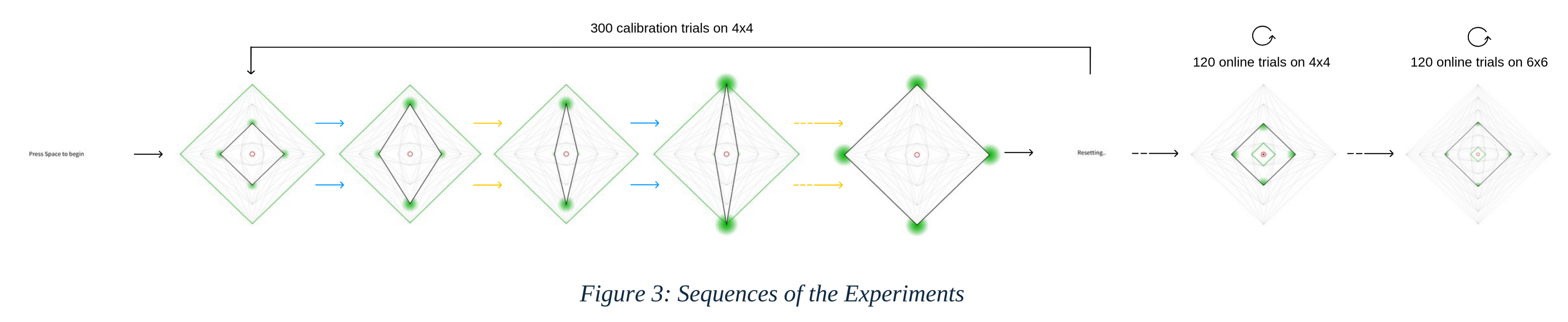
The shape in this study is used as the index rhombus is depicted in white (RGB: 255, 255, 255) and undergoes sequential changes in its dimensions, alternating between height and width in a width-height-width-height pattern. Each adjustment occurs in increments of one unit of the state space, with only one dimension being modified at a time. Once the index rhombus reaches its target position in one dimension, it proceeds to adjust the other dimension until it also attains its designated goal position. When both dimensions match with the goal or when threshold of the number of trials is met, it resets for a new block.
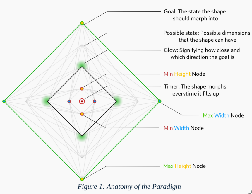
The state space represent all potential positions that the white rhombus can occupy. This feature is designed to inform subjects of the possible positions available during the task. The goal rhombus that signifies the target positions of the index rhombus is displayed in green (RGB: 0, 255, 0) and is randomly generated at the start of each block. It can be configured in four distinct ways: maximum height with maximum width, maximum height with minimum width, minimum height with maximum width, and minimum height with minimum width. A timer is visualized as a red circle that expands continuously at the very center of the screen. It resets after an interval of 3 seconds, serving as an anticipation cue for the movement. The movement of the index rhombus occurs when the circle reaches its maximum size, which is indicated by an unfilled stroked circle surrounding it. At each vertex of the rhombus, there is a glow that matches the color of the goal rhombus (green). This glow is always directed towards the goal and grows brighter as it approaches the target. The glow takes an elliptical shape, following the arc of the rhombus’s sides.
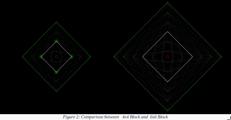
The experiment employs two distinct block configurations, 4×4 and 6×6, with their dimensions dynamically scaled according to the display height. To construct these blocks, the maximum size is set to 180% of the monitor height (calculated as 90% of the height, doubled), while the minimum size is set to 10% of the height (5% of the height, doubled). The range between these values is then divided into ten increments. Accordingly, the 4×4 blocks correspond to four increments of this division, while the 6×6 blocks correspond to six increments. Therefore, the possible sizes for the blocks in each dimension on a 1080p monitor would be 108, 291, 474, and 657 pixels for the 4×4 configuration, and additionally 840 and 1098 pixels for the 6×6 configuration.
The paradigm includes several screens to guide the user through the process: Begin, prompting “Press Space to start”; Reset, to reset the current state; Break, indicating a pause with the prompt “Take a Break. Press Space to Continue”; Break until instructed, a pause lasting until further instructions with the prompt “Take a Break… You will be instructed to continue soon.”; and “Finished”, marking the end of the experiment.
2.2 Experiment Setting #
2.2.1 Setup #
The EEG data were recorded using a ‘Brainvision 64-channel system’ with the signals amplified through an ‘Actichamp’ amplifier and the electrodes were applied using an ‘Actisnap’ cap. The visual stimuli were presented on an ‘ASUS VG279QM’ monitor, which features a resolution of 1080p, a refresh rate of 59.94Hz, and a 10-bit color depth in Standard Dynamic Range (SDR). The computational tasks were performed on a PC equipped with an ‘AMD Ryzen 5 5600G’ processor and 16GB of memory. A photodiode attached to the monitor was used for the assessment of any delays with the reception of stimulus and the markers pushed to the EEG data and a standard membrane keyboard used for the recording the responses. The software environment for the experiment comprised several key applications that played crucial roles in the research process. ‘Processing’ was employed to design and implement the experimental tasks (paradigm), allowing for real-time interaction with subjects. ‘Lab Streaming Layer’ (LSL) served as middleware, facilitating the real-time streaming of EEG data and ensuring seamless integration with the experimental software. ‘EEGLAB’ (Delorm & Makeig, 2004), a MATLAB toolbox, was utilized for the processing and analysis of EEG data, enabling advanced data manipulation and visualization. ‘BCILAB’ (Koethe et al., 2013) was used for the classification of EEG data through the LDA and windowed means approach, providing insights into the cognitive processes of the subjects. Finally, ‘SEREEGA’ (Krol et al., 2018) was instrumental in simulating various EEG data and creating the leadfield, as well as modeling and visualizing the spatial distribution of electrical activity in the brain.
The experiment was conducted in two distinct rooms: the ‘Control Room’ and the ‘EEG Room’. In the Control Room, subjects were prepared for the experiment, which included the application of the EEG cap. The experimenter monitored the subjects during this phase to ensure proper setup and comfort. The actual experimental trials took place in the EEG Room, which was dimly lit to minimize distractions and enhance subject focus.
2.2.2 Subjects #
Prior to participation, all subjects provided informed consent, ensuring they understood the nature of the study, the tasks involved, and their right to withdraw at any time. The study was conducted in accordance with ethical guidelines for research involving human subjects, and all procedures were approved by the Ethic Commission of Brandenburg University of Technology. A total of 19 subjects participated in this study, all of whom had normal or corrected-to-normal vision. The process of measuring head size and applying the EEG cap took up to one hour, ensuring that each subject was adequately prepared for the experiment. Subjects were seated comfortably in the Control Room prior to the commencement of the trials.
2.2.3 Instructions #
Subjects received detailed instructions regarding the experimental task. They were informed that a diamond shape, in this case the index rhombus, would morph periodically, alternating between width and height (i.e. in a sequence of width-height-width-height). A green diamond or the goal rhombus would be displayed on the screen, serving as the goal to which the diamond shape should morph towards. Subjects were instructed to evaluate whether the morphing diamond was moving closer to or away from the goal diamond with each shape change. To respond to the stimulus, they are to press ‘v’ on the keyboard if the shape morphs towards the goal or ‘b’ if the shape morphs away from the goal. Subjects were encouraged to respond as quickly as possible. If they were unsure or changed their mind, they could press the buttons again to correct their response. It was emphasized that subjects should press the button briefly and release it, avoiding the holding down of keys to prevent interference with the experiment. They were also asked to use only one hand to give the response. Whichever hand they may choose, must be used for the entire session.
The experiment included multiple breaks, which were announced on the screen. During these breaks, subjects had the opportunity to address any concerns or questions they may have had. They were also informed that if they needed to exit the experiment at any time, they could press the ‘ESC’ key, prompting the experimenter to assist with the removal of the EEG cap. Throughout the experiment, subjects were instructed to maintain a relaxed position, avoiding unnecessary movements or tension in their muscles. They were advised to notify the experimenter immediately if they experienced any discomfort or technical issues. To ensure optimal results, subjects were encouraged to stay focused on the task and minimize distractions.
2.2.4 Procedure #
The experimental procedure began with an orientation session, during which subjects were instructed on how to perform the task. Following this, they were left alone in the EEG Room and asked to start at their leisure. Initially, subjects completed 200 practice trials in a 4x4 experimental design, which were not included in the analysis. Subsequently, subjects engaged in 300 trials divided into three sets of 100 trials each, with breaks in between to reduce fatigue. After completing these trials, subjects were instructed to wait for further instructions while the experimenter trained the classifier using the recorded data. Once the training was complete, subjects resumed the task for the online phase at their leisure.
2.3 Classfication #
To analyze the brain’s electrical activity associated with the stimuli, event-related potentials (ERPs) were computed. This involved averaging the EEG data across multiple trials for each stimulus condition, enhancing the signal-to-noise ratio and revealing the underlying neural dynamics. The stimulus conditions here reflects the shape morphing towards the goal as ‘class1’ and away from the goal as ‘class2’. However, to minimize user error, trials where the subject gave wrong or multiple responses, were rejected. Hence, trials with only one and correct response were termed valid for the training of the classifier.
The EEG data was preprocessed to ensure signal integrity, which included resampling to a frequency of 100 Hz, re-referenced by average and band-pass filtered from 0.1 to 15 Hz. For feature extraction, BCILAB was used to segment the EEG data into epochs based on a predefined time range of 0 to 0.7 seconds surrounding the stimulus markers. Using the Windowed Means Approach (Blankertz et al., 2011) a window size of 50 milliseconds was established, resulting in a total of 14 discrete windows within the epoch. Classification was then proceeded by Linear Discriminant Analysis regularized by Shrinkage (Blankertz et al., 2011). For the reliability of the classification, a [5,5]-times nested cross-validation (Duda et al., 2001) with margins of 5 was used.
During the online phase for the open-loop experiment, the trained model was evaluated using the recorded test dataset. Recordings were acquired without applying the BCI (i.e., in the same manner as the calibration phase, with random movements). The test data underwent the same preprocessing pipeline as the training data, including relabeling to ensure label consistency. The model was then used to generate predictions, and performance was assessed by comparing the predicted labels with the true labels.
2.4 Implicit Control #
For the closed-loop experiment, the trained classifier was applied to control the morphing of a shape. Each morphing dimension (e.g., height and width) has an associated probability scale that ranges from −1 to 1 and is initialized at 0. On this scale, −1 denotes inward movement (towards the screen center) and +1 denotes outward movement (away from the screen center). When the classifier makes a prediction at the end of a move, the probability value for the corresponding dimension is adjusted by ±0.25 in the direction indicated by the prediction: an outward prediction increases the scale by +0.25, and an inward prediction decreases it by −0.25. For example, if the classifier predicts a movement ‘towards’ (class 1) when the shape morphed outward or away from the center for the height dimension, the height probability scale is increased by 0.25, making an outward move along the height more likely on the next move. Only predictions with confidence above 60% are applied to update the probability scales; lower-confidence predictions are ignored. During this online/test phase the classifier does not receive feedback about whether each prediction was correct, as it was receiving during the calibration phase. Updates were made regardless of the ground truth.
2.5 Post Hoc Analysis #
After the experiments, the recorded data was analyzed further by resampling to 250Hz and filtered by low cutoff frequency of 1Hz and rereferenced followed by Adaptive Mixture Independent Component Analysis (AMICA) of 2000 steps. Components that were identified and labeled as Eye and Muscle above the threshold of 0.85 by EEGLAB plugin - ICALabels were removed and pushed through the classification process to find out any difference between raw and clean data.
For Localization of the signal, we followed the methods of Krol et al. 2018, we combined the backward (LDA) spatial filter with independent component analysis (ICA). For each subject, the ICA unmixing matrix ( $W = [I_1, I_2, …, I_n]$ ) was computed on the cleaned data, such that $s = Wx$ ( $s$ are the component time courses and $x$ the sensor signals). For each analysis window, we assigned a relevance score $R_i$ to every independent component $I_i$ by mapping the LDA filter’s sensor weights into component space via $W$ and applying two multiplicative weighting terms. The first term adjusts for amplitude scaling between filter weights and component feature magnitudes: for component $i$ we compute the across-trial variance of its extracted feature $\hat F_i, V_i = var(\hat F_i)$ . The second term suppresses components unrelated to the task by scaling with the Pearson correlation between the component’s feature time series and the true class labels (as done previously at the electrode level). The resulting component relevance is therefore $R_i = V_i × corr(\hat F_i, L) × WM$ .
A standard ‘New York’ head model was used to create the leadfield with SEREEGA to identify equivalent dipole models that describe the likely position of the sources. This was accomplished using EEGLAB and its plugin DIPFIT 2.x. Components were selected based on a threshold criterion for residual variance (RV) of the dipole model (RV < 0.15) and through visual inspection of the activation spectra, time courses, and scalp topographies. Only dipolar components clearly reflecting cortical activity were included in the analysis, utilizing the cleaned data. For each time window, the resulting dipoles were weighted by the relevance Ri of their associated independent components. Areas of high relevance were then represented by a weighted dipole density plot using the EEGLAB plugin ‘dipoleDensity’. This plot displayed the dipole density per cubic millimeter, weighted by the relevance Ri of each included dipole, with a smoothing kernel of 12 mm.
We repeated the above training and classification procedure using trials with reduced distance to the goal and using single dimensions separately (width-only and height-only). The reduced-distance condition used trials two nodes away from the goal to test whether proximity increased signal strength; the index being close to the goal might reflect a higher valence for the morph, which could amplify the control signal. For the single-dimension analyses, trials for one dimension were selected only after the other dimension had reached its goal, allowing us to test whether one dimension produced a stronger signal than the other; this restriction was applied to reduce cognitive strain from subjects flip-flopping between dimensions, isolating the contribution of one dimension.
3. Results #
3.1 Calibration Phase #
With 19 participants involved in the study as subjects, the following table illustrates the outcomes regarding the number of trials each subject underwent in the respective classes during the calibration phase of the experiment, with the limit of 300 trials.
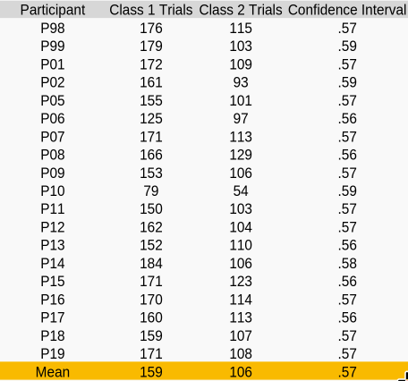
The paradigm was found to hav more class 1 trials than the class 2 , with class 1 trials having about 159 trials on average compared to 106 trials with class 2. Due to the non-uniform nature of the study, the confidence level was calculated using the stratified Wilson method of the fifth percentile. The average confidence interval across all subjects was determined to be 57.1%. The average user error rate calculated by the rejected trials being about 15.37%. Most subject’s EEG data consisted of high concentration of eye and muscle artifacts. Therefore, to evaluate the raw data - we chose P99 to be a suitable subject which consisted the least amount of above artifacts in its raw form. By raw we mean that the EEG data did not had its independent component removed but it did however went through the rereferencing, resampling, filtering procedure. Staying true to the analysis of Zander et al. (2016), we choose channel ‘Fz’ to investigate the signal and plotted spectral topographics with EEGLAB at the timestamps of 150, 200, 250, 300, 350, 400, 450, 500, 550ms.
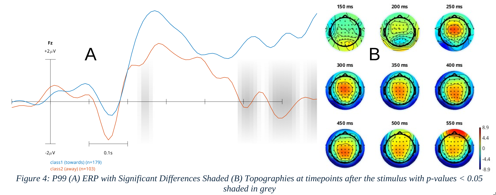
Analyzing the ERP, we find that the potential starts from a dip occuring at ~150ms after the stimulus. Similar to ICC, we notice one peak for the class 1 signal occuring at ~280ms. There are two peaks observed, first at ~210ms and the second at ~280ms for class 2. After the first peak of class 2, a difference between the two classes emerged, with the class 1 signal exhibiting a higher upward angular deviation compared to class 2. Consequently, the trough between the two peaks of class 2 showed a significant difference between the two classes (p<0.05) when performed a permutation test. With more significant differences found at the later timepoints, however likely due to the artifacts.
The topographies were plotted to show the occurences and the approximate location of dipoles. The topography at 150ms shows the development of the signal (contours at the front) with its visual counterpart (contours at the back), and then around 250ms clearly reflecting the occurrence of the developed signal concentrating at the channel ‘Cz’.
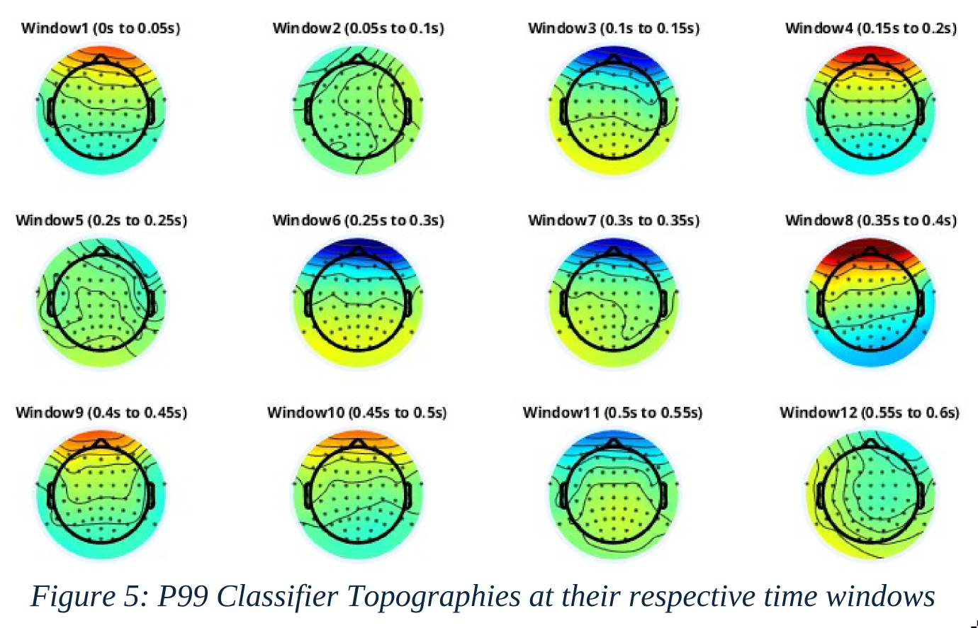
Coming to the classfications, visualizing the BCI results via BCILAB, we receive the topographies as shown in Fig 5. The classifier spectral topographies almost in all time windows were mostly covered with eye artifacts and this was prevalent among all subjects.
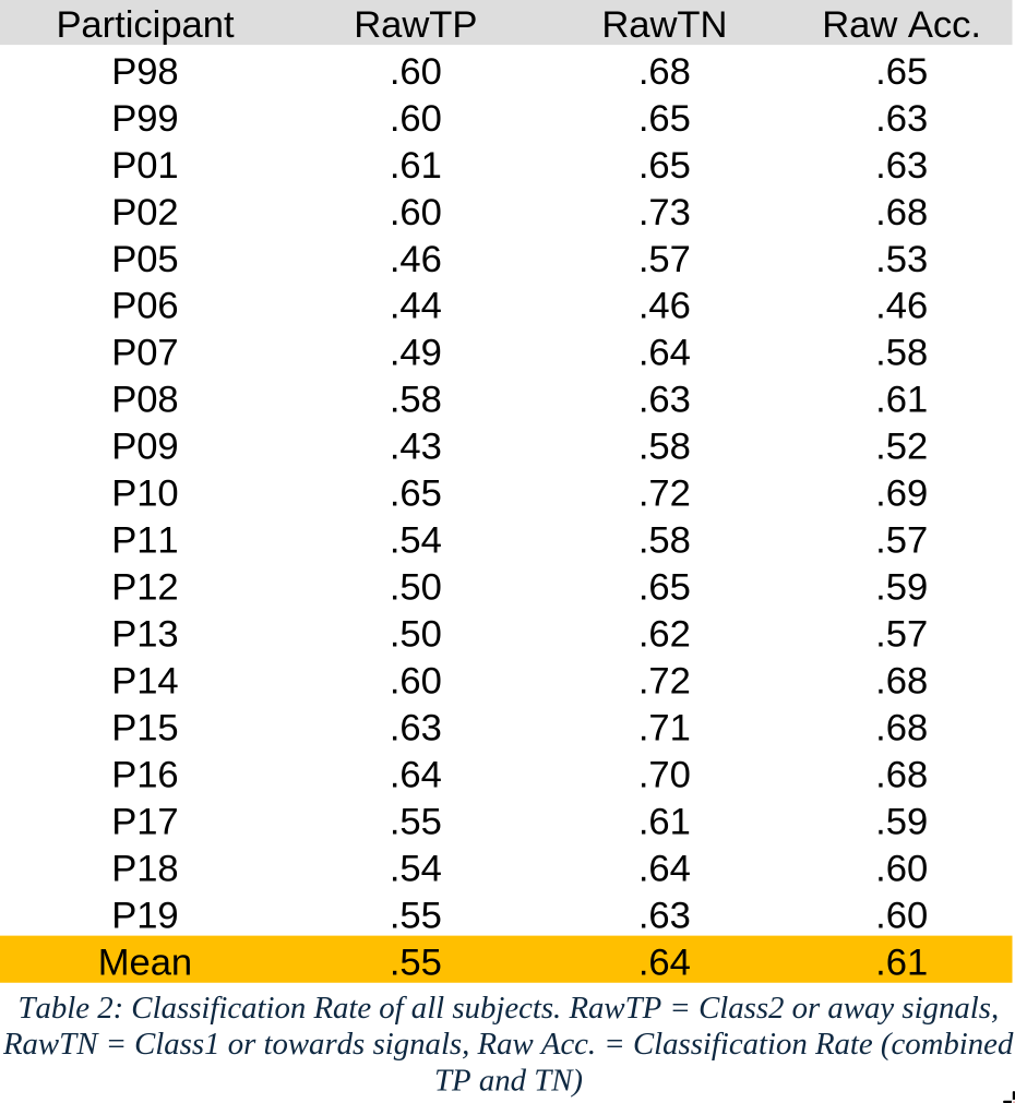
The mean accuracy of the 5 nested cross-validation (CV) test results stands at 60.6%(~61%), indicating a moderate level of predictive performance across the subjects. This average suggests that while the model demonstrates some capability in correctly classifying instances, there is considerable room for improvement. The highest accuracy recorded is 69.2%, achieved by subject P10. It is to be noted that the classifier was relied more on Class 1 as the true negatives (RawTN) is significantly higher than true positives (RawTP) or Class 2.
3.2 Online Phase #
In the online phase of the experiment, only 12 out of 19 subjects completed the closed-loop experiment. The following table presents the confusion matrix values for each subject at the end of the experiment, generated by the classifier’s predictions. As noted in the previous results, the classifier’s dependence on class 2 is further emphasized, as the true negatives (TN) are significantly higher than the other values.
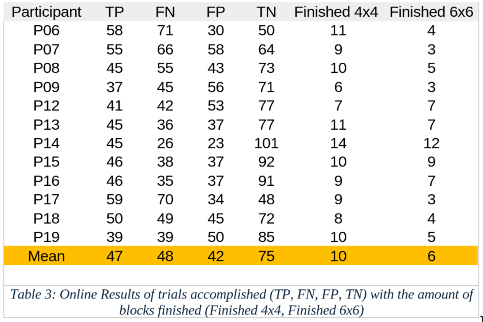
The closed-loop results reflects the calibration CV results with the class 1 trials having a higher classification rate in the online phase as well than the class 2. With P14 managing to accomplish 14 blocks of 4x4 and 12 blocks of 6x6.
When comparing the number of blocks completed by subjects over 120 trials for both the 4x4 and 6x6 configurations, we observe a normal distribution for both experiments with random moves. The results indicate that more blocks were cleared when the classifier was involved compared to when it was not.
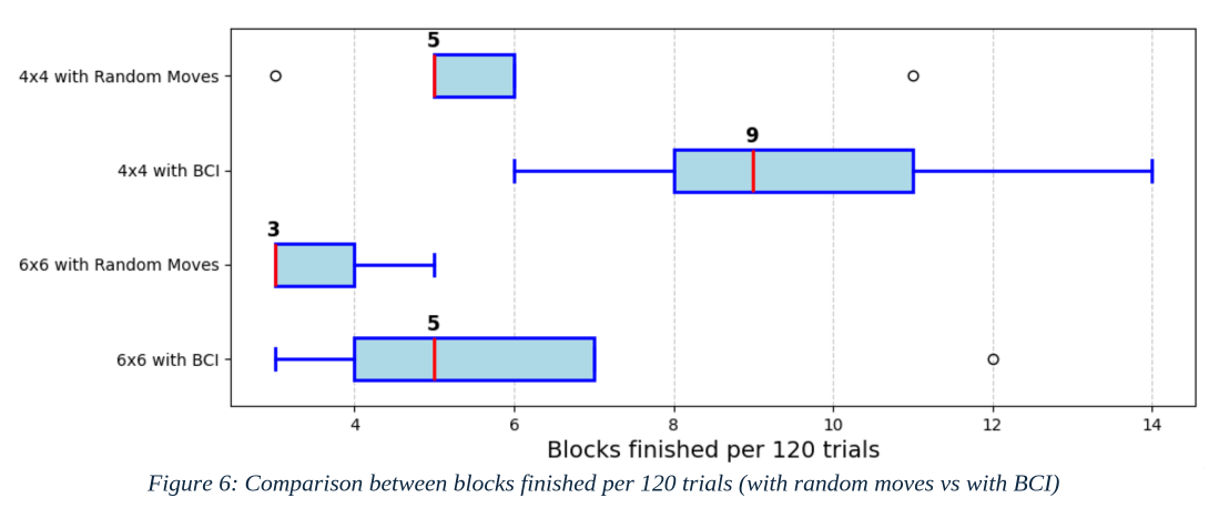
It is important to note that the sample size for both the 4x4 and 6x6 configurations with random moves was 100, while the sample size for the 4x4 and 6x6 configurations with BCI was 12, representing the number of subjects involved in closed-loop experiments. The median for 4x4 with random moves was 5, but 9 with BCI. For 6x6, it was 3 with random moves, but 5 with BCI. A Welch’s t-test was conducted to compare the performance of the experiments with random moves against those with BCI. The results indicated that the p- value for the 4x4 configuration was less than 0.001, while for the 6x6 configuration, it was less than 0.01.
3.3 Post-Hoc #
3.3.1 Grand Average #
Creating the Grand Average ERP with the raw data and cleaned data i.e. with the eye and muscle component removed, we discover how the components affected the variablity of the epochs.
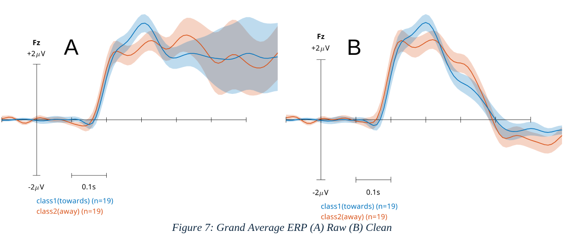
The grand average of the raw data denotes that the data stays consistent with the low variability atleast the control signal at 250ms but then comes higher variability following that around 300ms. The grandaverage of clean proves that those higher variablity was because of the eye and muscle components due to their absence.
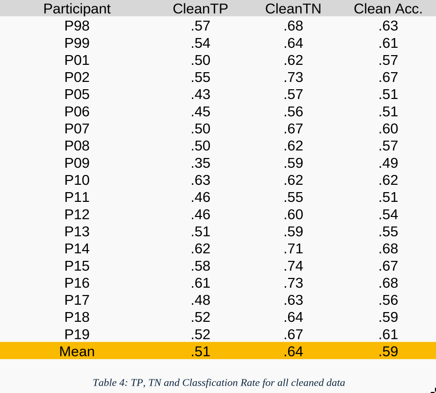
Performing the classification again, we arrive at the following results. The mean accuracy now being 58.9%(~59%) in average due to the lower accuracy from class 2 signal, however true negatives (cleanTN) remains constant with respect to raw data. This hints that there are other components must have minor impact on the classification for class 2 signals.
3.3.2 Localization #
The class co-related scalp activity using the LDA filter weights denoted the signal as in the following Fig.7 with the originating signal being assymetrical and mostly close to ‘FCz’ channel leaning posterior right.
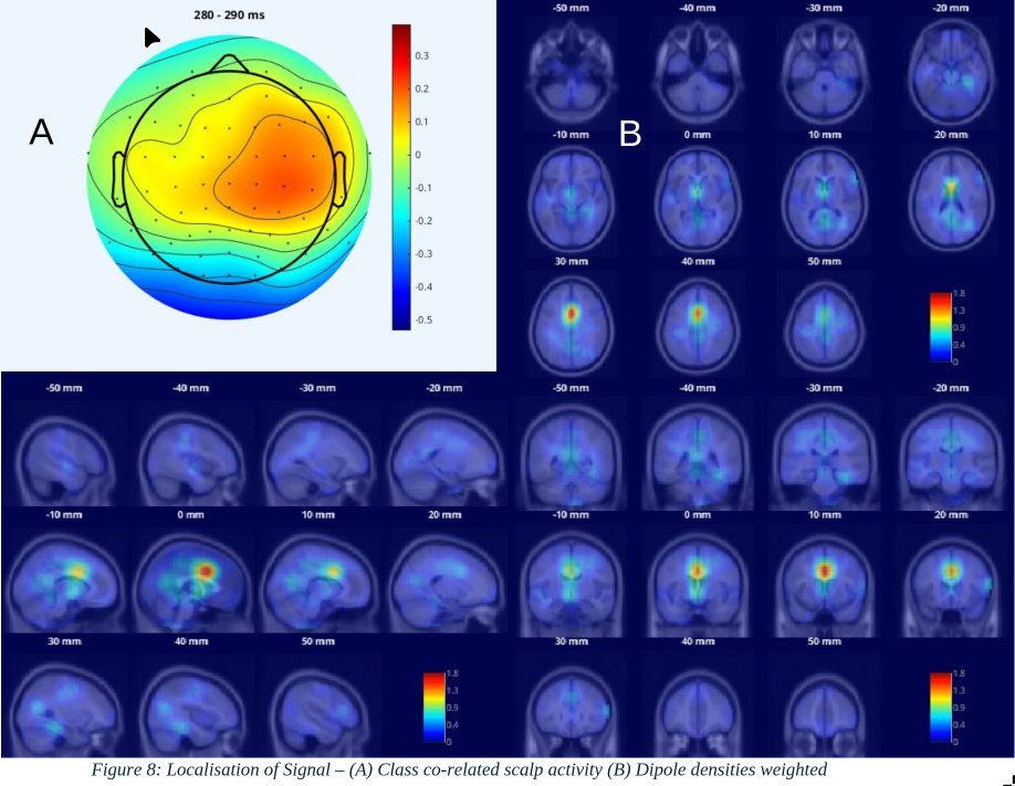
Localizing the signal with the density of the dipole, we are able to observe signal originating from Anterior Cingulate Cortex / Medial Prefrontal Cortex, right above the corpus callosum (0mm sagittal view) while being at the longitudinal fissure (30mm axial view). The top 5% dipoles (45) carry 42.32% of the weight.
3.3.3 Classification with Reduced Distance #
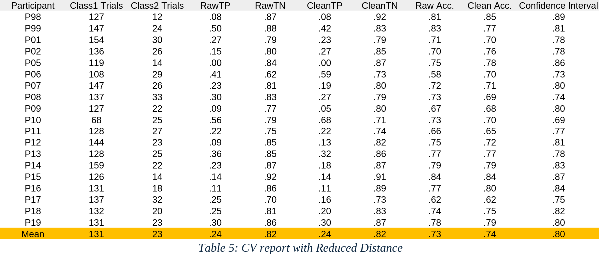
To find if the classification can be optimized by classifying the signals that are close to the goal, we do find that there is a greater difference between the trials and the accuracy for both raw and clean rises. Due to the higher difference between the number of trials, the confidence interval rises as well. With both rawTN and cleanTN being higher than the confidence interval in average and rawTP and cleanTP having much reduced classification rate.
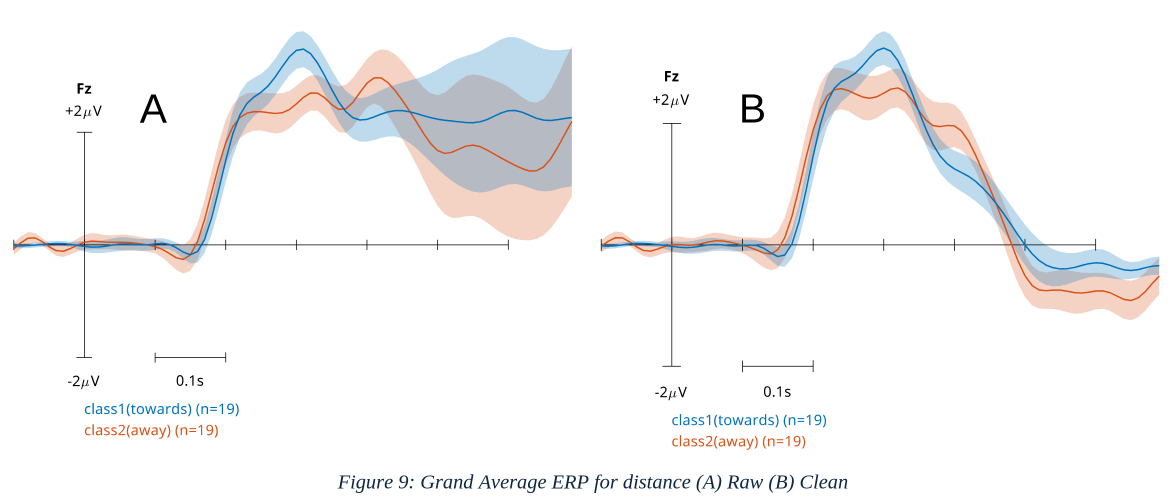
Plotting the ERP, we observe that the class 1 signal remains unchanged, however class 2 has a higher angular deviation and therefore a slight reduced second peak.
3.3.4 Classification with Single Dimensions #
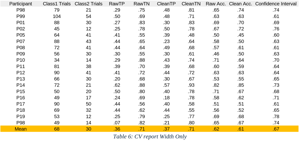
We find that there is 5% difference in average between the two dimensions for their classification rates (Raw Acc. & Clean Acc.). With TNs also having the same difference but TPs are higher in the height dimension.
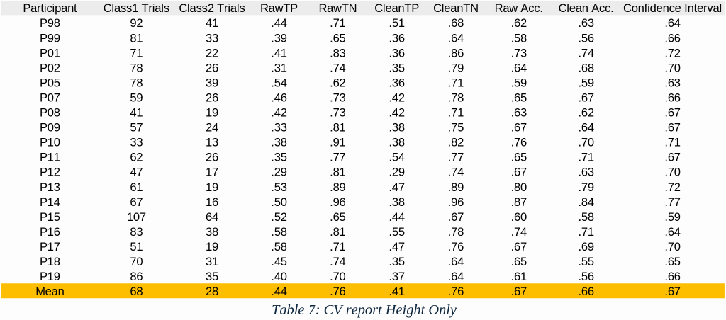
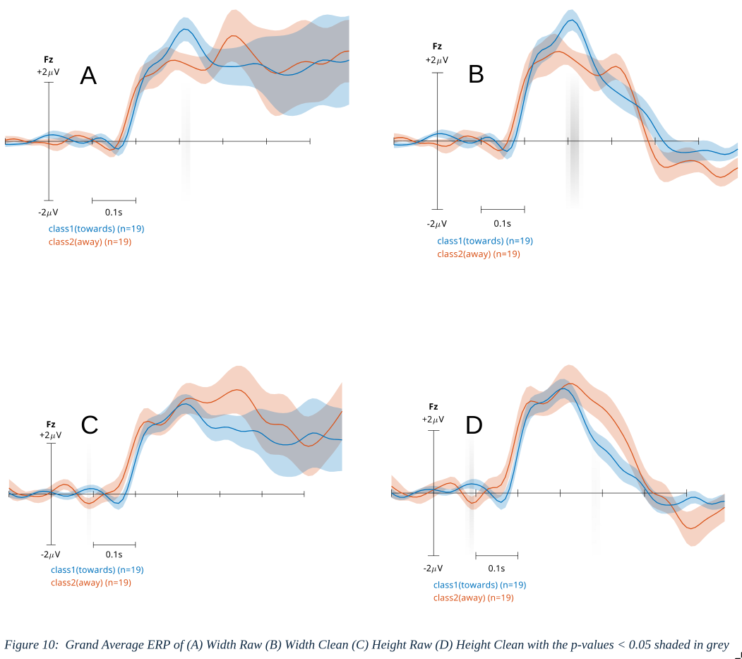
Plotting the ERPs, there is clear significant difference found around 300ms right at the peak for width only ERPs in both raw and clean data. However, none was found for height at the peak but only before the start of the peak around 90ms after the stimulus.
4. Discussion #
4.1 Interpretation #
The results convey that the paradigm produced a systematic bias of producing more trials of Class 1 than Class 2. The classification depends upon the ERP that emerges at Fz beginning ~150–200 ms post-stimulus with a peak near ~250 ms; this component served as the primary control signal used by the classifier [Table 1]. Across subjects, the classifier reliably detected this control signal to predict subjects’ intended morph direction when that intention corresponded to Class 1, but it failed to predict the opposite class above chance [Table 2]. In the online phase (120 trials per subject), subjects guided shapes to their target dimensions significantly more often than would be expected under random morphing [Figure 6]. Grand-average waveforms from both raw and ICA-cleaned data show the same ERP signature, although raw data contain additional variability after the peak consistent with eye and muscle artifacts [Figure 7]. This suggests the control signal is robust and not an artifact of preprocessing, and aggressive artifact removal may not be strictly necessary for reasonable classification. Performance on 6×6 (unseen) blocks — where glow/brightness cues were absent — remained above chance level, indicating subjects were not relying on simple brightness cues (glows) to drive decisions [Figure 2]. This generalization to unseen stimulus variants suggests the classifier may transfer to other paradigms that evoke similar error-related potentials.
Source localization and classifier topographies [Figure 8] indicate the control signal concentrates medially, consistent with mPFC activation (density of dipoles and classifier-based topography). This localization aligns with expected generators of error/expectation-violation signals and supports the interpretation that the detected ERP reflects cognitive evaluation relevant for morph-direction decisions.
Cross-validation analyses [Table 5] showed an increased imbalance in classification rates between Class 1 and Class 2 when distance (or separability) decreased; selecting trials with larger classifier distance/confidence improved class separation and overall accuracy. Reporting the distribution of classifier confidence and how thresholding affects both true positive and false positive rates will clarify the practical utility of such selection.
Classification accuracy was higher for width than for height [Table 6; Table 7]. A plausible explanation is greater temporal variability or weaker amplitude of the height-related ERP [Figure 10], reducing separability.
4.2 Limitations #
Subject motivation and engagement varied substantially and appeared to influence BCI performance: more motivated subjects generally achieved better control, introducing a potential confound with attention and effort (Kleih et al., 2010). Because we did not systematically measure motivation as a covariate, its effect on results remains uncertain and should be controlled or recorded in future work.
The study took place in a non-soundproof room, so uncontrolled environmental noise and interruptions may have increased cognitive load and reduced BCI effectiveness for some subjects. Relatedly, delays during electrode gel application lengthened sessions and increased fatigue; subjects reporting longer gelling times tended to perform worse, suggesting session logistics affected attentional resources and data quality.
Several stimulus design issues likely affected subject experience and data. The growing red circle animation was reported as distracting or soporific by some subjects, and many found the rhombus growth stages too fast, which may have induced drowsiness or pressured rapid responses. Additionally, a height–width perceptual illusion was observed: changes to one dimension sometimes produced a perceived change in the other, potentially confusing subjects and contaminating behavioural measures.
No subjects were excluded from analysis; all subjects and their recorded sessions were retained. As a result, several figures and summary statistics include data with substantial artifacts, and low-quality recordings from a subset of subjects whose signals were not reliably retrieved. Retaining all subjects preserves sample size and avoids bias from selective exclusion, but it increases noise in group averages, inflates variance estimates, and can obscure true effects—particularly for measures sensitive to single-trial quality (e.g., ERPs and classifier performance). Because no objective, pre-registered criteria for trial or subject exclusion were applied, the reported group-level results should be interpreted as reflecting performance under pragmatic, inclusive data handling rather than optimal cleaned datasets. Future work should predefine artifact and subject-rejection criteria (for example: minimum channel yield, baseline SNR threshold, maximum proportion of rejected trials), report results both with and without excluded sessions, and consider robust statistics or weighted analyses that down-weight low-quality recordings to balance inclusivity with data fidelity.
Analytical limitations include the restricted state-space used for reduced-distance analyses (4×4), which provides insufficient coverage to fully characterise how morph distance affects the control signal; higher-dimensional blocks and more trials per condition are needed to draw stronger conclusions. We also observed greater ERP variability for height trials than for width trials, reducing classification accuracy for height; the source of this asymmetry is unknown and requires targeted follow-up (e.g., single-trial SNR, latency variance, and time–frequency comparisons). Finally, subject frustration emerged when shapes repeatedly morphed in the wrong direction due to near-chance “away” signals. This negative feedback likely reduced engagement and could have impaired learning or performance across blocks. Future studies should mitigate these issues via improved lab control, streamlined setup, stimulus adjustments, better measurement of motivation/engagement, larger state spaces, and adaptive feedback strategies.
4.3 Comparisons #
The primary conceptual difference is target geometry: ICC concerns object location (where a cursor is relative to a goal), whereas ISMC concerns object size (how an object’s dimensions change toward a goal). That shift alters the user’s mental computations and the task affordances: location control is a single spatial vector problem, while size control requires assessing distances along object edges or dimensions, which can add cognitive load and change the kinds of perceptual cues that drive neural responses. In ICC users typically compute a single distance or directional error from the cursor to the goal — a straightforward spatial judgment. In ISMC, users must evaluate distances from one or both sides of a shape (e.g., left/right for width, top/bottom for height) to the target dimension; practically this is more like judging two margins rather than one offset. This binary/dual-sided nature can complicate decision-making and may explain why ISMC produced more “towards” trials than “away” trials in our data: subjects may bias the system toward corrective (toward-goal) signals when confronted with ambiguous size cues.
ICC typically offers more movement alternatives (in our reference ICC implementation there are eight possible cursor directions), giving a richer, higher-dimensional action space. ISMC used essentially binary choices per dimension (increase vs. decrease), reducing the output space to low dimensionality (analogous to repeated coin tosses). This lower degree of freedom affects both user strategy and classifier demands: with fewer discrete outcomes, classifiers must discriminate subtler differences in the same ERP signature across fewer labels, and users may adopt simpler corrective heuristics.
Topographies and source estimates suggest the ISMC control signal is concentrated spherically and more medially, just above the corpus callosum , whereas ICC signals in prior work shows a broader or elongated oval dipole that include regions nearer to the corpus callosum.
4.4. Future Scope #
Future work should prioritize reducing cognitive load by simplifying task demands. Limiting the number of response options and streamlining trial structure (shorter trials, fewer simultaneous choices) can reduce decision time, lower error rates, and help subjects maintain consistent performance across sessions, as Wolpaw et al. (2002) and Mak & Wolpaw (2009) emphasize the importance of ergonomic task design for reliable BCI control. Empirical work on user training and workload by Faller et al. (2019) further supports shorter, focused trials to prevent fatigue and accelerate learning; accordingly, trial-level adjustments should be systematically evaluated to balance efficiency and classifier robustness.
Enhancing visual clarity and spatial cues will likely improve subject understanding and accuracy. Increasing node salience (contrast, size, labeling), adding brief instructional highlights of node-to-node relationships, or overlaying subtle gridlines can help subjects form clearer mental maps and perform spatial calculations with less effort. This approach aligns with human–computer interaction findings on perceptual salience and task performance (Zander et al., 2016) and with studies showing that clearer stimulus representations reduce inter- and intra-subject variability in EEG-based tasks (Saha & Baumert, 2020).
Integrating dynamic, multimodal feedback can accelerate learning and sustain engagement. Animated representations of the rhombus expanding or contracting provide immediate, intuitive progress signals; complementary adaptive color gradients, morphing audio cues, or movement-based displays (e.g., clock-like rotational paradigms) create redundant channels so users can rely on the modality that best matches their cognitive style. Lotte et al. (2018) review multimodal and adaptive feedback strategies for BCI training, and neuroadaptive frameworks proposed by Zander and colleagues (2016) highlight the value of aligning feedback modalities with implicit and explicit cognitive states to improve control.
Reframing task goals—such as testing a “danger zone” (avoidance) paradigm instead of a single attractor—may reveal different control strategies and improve transfer to applied tasks. Avoidance-based framing can encourage alternative behaviors and clarify task dynamics for some subjects; Chavarriaga and Millán (2010) and Blankertz et al. (2008) indicate that different task framings and error-related signals can change the neural correlates available for decoding. Within-subject comparisons of approach versus avoidance framings will help determine which yields faster learning, greater robustness, and lower subjective workload.
Calibration and classifier strategies warrant systematic exploration to reduce setup time while maintaining performance. Shorter calibration phases and trials with reduced distances may increase efficiency but require evaluation for impacts on classifier robustness. Online adaptive classification that updates with incoming EEG can shorten effective calibration by reaching an acceptable accuracy threshold sooner; Vidaurre et al. (2011) and Wu et al. (2020) describe adaptive and transfer-learning approaches that reduce calibration needs. Hybrid strategies—pretraining a universal classifier on group-level data and fine-tuning it online for each subject—combine generalization with personalization and have been shown to improve initial performance and reduce training time (Lotte et al., 2018; Wu et al., 2020). Investigating a full paradigm shift—systematically comparing current goal/approach-based designs with novel paradigms such as danger-zone framing, rotational/motion-based interfaces, or narrative-driven tasks—will clarify which paradigms best support rapid calibration, robust control, and generalization across users.
Personalization of feedback and difficulty is likely to improve learning and retention. Adaptive algorithms that adjust target tolerance, feedback salience, cue modality, or difficulty pacing based on individual performance trajectories keep tasks challenging but attainable. Faller et al. (2019) outline training-method frameworks that adapt to subject learning curves, while Saha and Baumert (2020) document how intra- and inter-subject variability necessitates individualized calibration and feedback to achieve stable control.
Motivation and reward structures can increase engagement and clarify control drivers. Implementing scoring systems, progress indicators, or small monetary incentives may sustain attention across sessions and help distinguish whether control signals are primarily affective (reward-driven) or analytical (strategy-driven). Wolpaw and colleagues’ clinical and translational discussions (Mak & Wolpaw, 2009; Wolpaw et al., 2002) and studies of implicit reward signals in neuroadaptive systems (Zander et al., 2016) suggest experimental comparisons of incentivized versus non-incentivized conditions to quantify motivational effects on performance and neural signatures.
Expanding the range of paradigms and sensory mappings will help identify approaches that generalize across populations. Beyond visual and auditory modalities, consider haptic feedback, symbolic metaphors, or narrative-driven tasks that may be more intuitive for specific user groups. Reviews by Nicolas-Alonso and Gomez-Gil (2012) and Lotte et al. (2018) catalog a variety of stimulus and feedback paradigms; systematic testing across demographic and clinical groups will indicate which mappings maximize usability and transfer.
Finally, combined studies should measure objective performance (accuracy, throughput), learning curves, subjective workload, and retention to guide pragmatic design decisions. Integrating robust classifier methods (Blankertz et al., 2008), adaptive/online training (Vidaurre et al., 2011; Wu et al., 2020), pretrained universal classifiers fine-tuned online (Lotte et al., 2018), and user-centered feedback strategies (Faller et al., 2019; Zander et al., 2016) will help make the BCI paradigm faster to calibrate, easier to use, and more robust across subjects, improving both experimental outcomes and real-world applicability.
5. Conclusion #
This thesis demonstrates a proof-of-principle for implicit shape-morph control using EEG-decoded expectation-violation/error-related potentials. Across 19 subjects (12 in closed-loop), a shrinkage-regularized LDA trained on windowed ERP features decoded morph-direction signals above chance (mean nested-CV raw ≈ 61%; cleaned ≈ 59%) and produced behaviorally meaningful effects in the online phase: subjects completed significantly more blocks with the BCI than with random morphing (4×4: p < 0.001; 6×6: p < 0.01). The primary discriminative ERP emerged at frontocentral electrodes beginning ~150– 200 ms and peaking near ~250–300 ms, and source/dipole-density analyses localized the signal medially, consistent with mPFC/ACC generators implicated in expectancy violation and performance monitoring.
While these outcomes support the central hypothesis that passive evaluative ERPs can bias continuous visual morphing toward user goals, performance was moderate and asymmetrical. Class-imbalance in the paradigm (more Class-1/toward trials), pervasive ocular/myogenic artifacts, and per-subject variability constrained classifier reliability—particularly for “away” (Class-2) decoding. Reduced-distance trials and single-dimension analyses indicated improved separability and a modest (~5%) advantage for height over width decoding, but the height condition also showed greater temporal variability. These findings suggest the control signal is robustly cortical yet sensitive to task framing, perceptual cues, and data quality.
In sum, EEG-decoded expectancy-violation signals—centered on mPFC—provide a viable low-dimensional implicit control channel for shape morphing. With methodological refinements (better calibration strategies, artifact control, and user-centered design), this paradigm can scale toward more reliable, expressive neuroadaptive interfaces for hands-free design, gaming, and VR applications.
6. References #
Abdulkader, S. N., Atia, A., & Mostafa, M. S. (2015). Brain computer interfacing: Applications and challenges. Egyptian Informatics Journal, 16(2), 213–230. https://doi.org/10.1016/j.eij.2015.04.011
Blankertz, B., Lemm, S., Treder, M., Haufe, S., & Müller, K.-R. (2011). Single-trial analysis and classification of ERP components — A tutorial. NeuroImage, 56(2), 814–825. Blankertz, B., Tomioka, R., Lemm, S., Kawanabe, M., and Muller, K. -r. (2008).
“Optimizing Spatial filters for Robust EEG Single-Trial Analysis” in IEEE Signal Processing Magazine, vol. 25, no. 1, pp. 41-56, 2008, doi: 10.1109/MSP.2008.4408441
Chavarriaga R, Millan Jdel R. Learning from EEG error-related potentials in noninvasive brain-computer interfaces. IEEE Trans Neural Syst Rehabil Eng. 2010 Aug;18(4):381-8. doi: 10.1109/TNSRE.2010.2053387. Epub 2010 Jun 21. PMID: 20570777.
Delorme, A., & Makeig, S. (2004). EEGLAB: an open source toolbox for analysis of single- trial EEG dynamics including independent component analysis. Journal of Neuroscience Methods, 134(1), 9–21.
Duda, R. O., Hart, P. E., & Stork, D. G. (2001). Pattern Classification (2nd ed.). Wiley. https://www.researchgate.net/publication/228058014_Pattern_Classification
Esteva, A., Robicquet, A., Ramsundar, B., Kuleshov, V., DePristo, M., Chou, K., … & Dean, J. (2019). A guide to deep learning in healthcare. Nature Medicine, 25(1), 24–29. https://doi.org/10.1038/s41591-018-0316-z
Faller J, Cummings J, Saproo S, Sajda P. Regulation of arousal via online neurofeedback improves human performance in a demanding sensory-motor task. Proc Natl Acad Sci U S A. 2019 Mar 26;116(13):6482-6490. doi: 10.1073/pnas.1817207116. Epub 2019 Mar 12. Erratum in: Proc Natl Acad Sci U S A. 2019 Apr 9;116(15):7598. doi: 10.1073/pnas.1904484116. PMID: 30862731; PMCID: PMC6442591.
Gomez-Uribe, C. A., & Hunt, N. (2016). The Netflix recommender system: Algorithms, business value, and innovation. ACM Transactions on Management Information Systems, 6(4), Article 13. https://doi.org/10.1145/2843948
Goodall, N. J. (2014). Machine ethics and automated vehicles. In G. Meyer & S. Beiker (Eds.), Road Vehicle Automation (Vol. 2, pp. 93–102). Springer. https://doi.org/10.1007/978- 3-319-05990-7_8
Hajcak, G., MacNamara, A., & Olvet, D. M. (2010). Event-related potentials, emotion, and emotion regulation: An integrative review. Developmental Neuropsychology, 35(2), 129–155. https://doi.org/10.1080/87565640903526504
Jeannerod, M. (1994). The representing brain: Neural correlates of motor intention and imagery. Behavioral and Brain Sciences, 17(2), 187–202. https://doi.org/10.1017/S0140525X00034020
Kleih SC, Nijboer F, Halder S, Kübler A. Motivation modulates the P300 amplitude during brain-computer interface use. Clin Neurophysiol. 2010 Jul;121(7):1023-31. doi:10.1016/j.clinph.2010.01.034. Epub 2010 Feb 25. PMID: 20188627.
Kosslyn, S. M., Ganis, G., & Thompson, W. L. (2001). Neural foundations of imagery. Nature Reviews Neuroscience, 2(9), 635–642. https://doi.org/10.1038/35090055
Kothe, C. A., Vergotte, G., Mullen, T., Bigdely-Shamlo, N., & Kreutz-Delgado, K. (2013). BCILAB: A platform for brain–computer interface development. Journal of Neural Engineering, 10(5), 056014.
Krol, L., Mousavi, M., De Sa, V., & Zander, T. (2018). Towards Classifier Visualisation in 3D Source Space. 2018 IEEE International Conference on Systems, Man, and Cybernetics (SMC), 71–76. https://doi.org/10.1109/SMC.2018.00022
Krol, L. R., Pawlitzki, J., Mousavi, M., Andreessen, L. M., & Zander, T. O. (2019). Salience versus Valence in Implicit Cursor Control: First Indications of Separate Cortical Processes. In 2019 IEEE International Conference on Systems, Man and Cybernetics (SMC) (pp. 3913– 3918). https://doi.org/10.1109/SMC.2019.8913936
Krol, L. R., van de Vel, A., de Boer, M., van der Kamp, J., & Putten, M. J. A. M. van (2018). SEREEGA: Simulating event-related EEG activity. Journal of Open Source Software, 3(24), 635.
Lotte, F., Bougrain, L., Cichocki, A., Clerc, M., Congedo, M., Rakotomamonjy, A., & Yger, F. (2018). A review of classification algorithms for EEG-based brain–computer interfaces: A 10 year update. Journal of Neural Engineering, 15(3), 031005. https://doi.org/10.1088/1741- 2552/aab2f2
Oostenveld, R., Fries, P., Maris, E., & Schoffelen, J.-M. (2011). FieldTrip: Open source software for advanced analysis of MEG, EEG, and invasive electrophysiological data. Computational Intelligence and Neuroscience, 2011, 156869.
Lebedev, M. A., & Nicolelis, M. A. L. (2006). Brain–machine interfaces: Past, present and future. Trends in Neurosciences, 29(9), 536–546. https://doi.org/10.1016/j.tins.2006.07.004
Nicolas-Alonso, L. F., & Gomez-Gil, J. (2012). Brain computer interfaces, a review. Sensors, 12(2), 1211–1279. https://doi.org/10.3390/s120201211
Olofsson, J. K., Nordin, S., Sequeira, H., & Polich, J. (2008). Affective picture processing: An integrative review of ERP findings. Biological Psychology, 77(3), 247–265. https://doi.org/10.1016/j.biopsycho.2007.11.006
Pfurtscheller, G., & Neuper, C. (2001). Motor imagery and direct brain–computer communication. Proceedings of the IEEE, 89(7), 1123–1134. https://doi.org/10.1109/5.939829
Saha S, Baumert M. Intra- and Inter-subject Variability in EEG-Based Sensorimotor Brain Computer Interface: A Review. Front Comput Neurosci. 2020 Jan 21;13:87. doi: 10.3389/fncom.2019.00087. PMID: 32038208; PMCID: PMC6985367.
Schupp, H. T., Flaisch, T., Stockburger, J., & Junghöfer, M. (2006). Emotion and attention: Event-related brain potential studies. Progress in Brain Research, 156, 31–51.
Shaker, N., Togelius, J., & Nelson, M. J. (2016). Procedural Content Generation in Games. Springer. https://doi.org/10.1007/978-3-319-42711-1
Vidaurre, C.; Kawanabe, M.; von Bünau, P.; Blankertz, B.; Müller, K. R., “Toward unsupervised adaptation of LDA for brain–computer interfaces”, IEEE Trans. Biomed. Eng., vol. 58, no. 3, pp. 587–597, Mar. 2011, doi: 10.1109/TBME.2010.2093133.
Wolpaw, J. R., Birbaumer, N., McFarland, D. J., Pfurtscheller, G., & Vaughan, T. M. (2002). Brain–computer interfaces for communication and control. Clinical Neurophysiology, 113(6), 767–791. https://doi.org/10.1016/S1388-2457(02)00057-3
Wolpaw, J. R., & Wolpaw, E. W. (Eds.). (2012). Brain–Computer Interfaces: Principles and Practice. Oxford University Press.
Wu, D.; Xu, Y.; Lu, B.-L., “Transfer learning for EEG-based brain–computer interfaces: A review of progress made since 2016,” IEEE Trans. Cogn. Dev. Syst., vol. 14, no. 1, pp. 4–19, Mar. 2022, doi: 10.1109/TCDS.2020.3007453
Zander, T. O., & Kothe, C. (2011). Towards passive brain–computer interfaces: Applying BCI technology to human–machine systems in general. Journal of Neural Engineering, 8(2), 25005. https://doi.org/10.1088/1741-2560/8/2/025005
Zander, T. O., Krol, L. R., Birbaumer, N., & Gramann, K. (2016). Neuroadaptive technology for implicit cursor control based on medial prefrontal cortex activity. Neuroinformatics, 14(3), 301–313. doi:10.1007/s12021-016-9320-1